Perceptual Losses for Real-Time Style Transfer and Super-Resolution
ECCV 2016,实时风格迁移与超分辨率化的感知损失,这篇论文是在cs231n里面看到的,正好最近在研究风格迁移。一作是Justin Johnson,2017春的cs231n的主讲之一。这篇论文的主要内容是对Gatys等人的风格迁移在优化过程中进行了优化,大幅提升了性能。
主要原理就是,之前Gatys等人的论文是利用已经训练好的VGG19,求loss并利用VGG的结构反向求导更新图片。由于VGG结构复杂,这样反向更新速度很慢,改进方法是再另外设计一个神经网络,将内容图片作为输入,输出扔到VGG中做两个loss,然后反向传播更新当前这个神经网络的参数,这样训练出来的神经网络就可能将任意的内容图片扔进去,输出为风格迁移后的图片,这也就解决了速度的问题。这也就是将Feed-forward image transformation与style transfer结合在一起。原文链接:Perceptual Losses for Real-Time Style Transfer and Super-Resolution
Image Transformation Network
Architecture
We do not use any pooling layers, instead using strided and fractionally strided convolutions for in-network downsampling and upsampling. Our network body consists of five residual blocks using the architecture of http://torch. ch/blog/2016/02/04/resnets.html. All non-residual convolutional layers are followed by spatial batch normalization and ReLU nonlinearities with the exception of the output layer, which instead uses a scaled tanh to ensure that the output image has pixels in the range [0, 255]. Other than the first and last layers with use $9 \times 9$ kernels, all convolutional layers use $3 \times 3$ kernels. The exact architectures of all our networks can be found in the supplementary material.
Inputs and Outputs
For style transfer the input and output are both color images of shape #3 \times 256 \times 256#.
For super-resolution with an upsampling factor of $f$, the output is a high-resolution patch of shape $3 \times 288/f \times 288/f$. Since the image transformation networks are fully-convolutional, at test-time they can be applied to images of any resolution.
Downsampling and Upsampling
For super-resolution with an upsampling factor of $f$, we use several residual blocks followed by $log_2f$ convolutional layers with stride $1/2$. This is different from [1] who use bicubic interpolation to upsample the low-resolution input before passing it to the network.
Our style transfer networks use the architecture shown in Table 1 and our super-resolution networks use the architecture shown in Table 2. In these tables “$C \times H \times W$ conv” denotes a convolutional layer with $C$ filters size $H \times W$ which is immeidately followed by spatial batch normalization [1] and a ReLU nonlinearity.
Our residual blocks each contain two $3 \times 3$ convolutional layers with the same number of filters on both layer. We use the residual block design of Gross and Wilber [2] (shown in Figure 1), which differs from that of He et al [3] in that the ReLU nonlinearity following the addition is removed; this modified design was found in [2] to perform slightly better for image classification.
For style transfer, we found that standard zero-padded convolutions resulted in severe artifacts around the borders of the generated image. We therefore remove padding from the convolutions in residual blocks. A $3 \times 3$ convolution with no padding reduces the size of a feature map by 1 pixel on each side, so in this case the identity connection of the residual block performs a center crop on the input feature map. We also add spatial reflection padding to the beginning of the network so that the input and output of the network have the same size.
Perceptual Loss Functions
We define two perceptual loss functions that measure high-level perceptual and semantic differences between images. They make use of a loss network $\phi$ pretrained for image classification, meaning that these perceptual loss functions are themselves deep convolutional neural networks. In all our experiments $\phi$ is the 16-layer VGG network pretrained on the ImageNet dataset.
Featue Reconstruction Loss
Rather than encouraging the pixels of the output image $\hat{y} = f_W(x)$ to exactly match the pixels of the target image $y$, we instead encourage them to have similar feature representations as computed by the loss network $\phi$. Let $\phi_j(x)$ be the activations of the jth layer of the network $\phi$ when processing the image $x$; if $j$ is a convolutional layer then $\phi_j(x)$ will be a feature map of shape $C_j \times H_j \times W_j$. The feature reconstruction loss is the (squared, normalized) Euclidean distance between feature representations:
As demonstrated in [6] and reproduced in Figure 3, finding an image $\hat{y}$ that minimizes the feature reconstruction loss for early layers tends to produce images that are visually indistinguishable from $y$.
Style Reconstruction Loss
The feature reconstruction loss penalizes the output image $\hat{y}$ when it deviates in content from the target $y$. We also wish to penalize differences in style: colors, textures, common patterns, etc. To achieve this effect, Gatys et al propose the following style reconstruction loss.
As above, let $\phi_j(x)$ be the activations at the $j$th layer of the network $\phi$ for the input $x$, which is a feature map of shape $C_j \times H_j \times W_j$. Define the Gram matrix $G^\phi_j(x)$ to be the $C_j \times C_j$ matrix whose elements are given by
Experiments
Style Transfer
Single-Image Super_Resolution
This is an inherently ill-posed problem, since for each low-resolution image there exist multiple high-resolution images that could have generated it. The ambiguity becomes more extreme as the super-resolution factor grows; for larger factors ($\times 4$, $\times 8$), fine details of the high-resolution image may have little or no evidence in its low-resolution version.
To overcome this problem, we train super-resolution networks not with the per-pixel loss typically used [1] but instead with a feature reconstruction loss to allow transer of semantic knowledge from the pretrained loss network to the super-resolution network. We focus on $\times 4$ and $\times 8$ super-resolution since larger factors require more semantic reasoning about the input.
The traditional metrics used to evaluate super-resolution are PSNR and SSIM, both of which have been found to correlate poorly with human assessment of visual quality. PSNR and SSIM rely only on low-level differences between pixels and operate under the assumption of additive Gasussian noise, which may be invalid for super-resolution. In addition, PSNR is equivalent to the per-pixel loss $\mathcal{l_{pixle}}$, so as measured by PSNR a model trained to minimize feature reconstruction loss should always outperform a model trained to minimize feature reconstruction loss. We therefore emphasize that the goal of these experiments is not to achieve state-of-the art PSNR or SSIM results, but instead to showcase the qualitative difference between models trained with per-pixel and feature reconstruction losses.
code
我用gluon实现了一个2x的超分辨率网络,训练后感觉效果一般,只有一次loss降到了40附近,那次效果挺好,但是颜色并不是很好
以下是代码:1
2
3
4
5
6
7
8
9
10
11
12
13
14
15
16
17
18
19
20
21
22
23
24
25
26
27
28
29
30
31
32
33
34
35
36
37
38
39
40
41
42
43
44
45
46
47
48
49
50
51
52
53
54
55
56
57
58
59
60
61
62
63
64
65
66
67
68
69
70
71
72
73
74
75
76
77
78
79
80
81
82
83
84
85
86
87
88
89
90
91
92
93
94
95
96
97
98
99
100
101
102
103
104
105
106
107
108
109
110
111
112
113
114
115
116
117
118
119
120
121
122
123
124
125
126
127
128import mxnet as mx
from mxnet import nd
import numpy as np
import os
from mxnet import autograd
from mxnet import gluon
from mxnet.gluon import nn
from mxnet import init
from mxnet.gluon.model_zoo import vision as models
import matplotlib.pyplot as plt
# get_ipython().run_line_magic('matplotlib', 'inline')
import logging
logger = logging.getLogger(__name__)
data_filenames = ['trainx_%s.params'%(i) for i in range(7)]
target_filenames = ['trainy_%s.params'%(i) for i in range(7)]
load_params = True
epochs = 500
batch_size = 4
ratio = 0.1
learning_rate = 1e-5
start_index, end_index = 0, 7
num_samples = end_index - start_index
ctx = [mx.gpu(i) for i in range(1)]
if load_params == False:
with open('training.log', 'w') as f:
f.write('')
class residual_unit(gluon.HybridBlock):
def __init__(self, channels, **kwargs):
super(residual_unit, self).__init__(**kwargs)
self.conv1 = nn.Conv2D(channels = channels, padding=1, kernel_size=3, strides=1, use_bias=False)
self.bn1 = nn.BatchNorm(momentum=0.9)
self.act1 = nn.Activation('relu')
self.conv2 = nn.Conv2D(channels = channels, padding=1, kernel_size=3, use_bias=False)
self.bn2 = nn.BatchNorm(momentum=0.9)
self.act2 = nn.Activation('relu')
self.conv3 = nn.Conv2D(channels = channels, kernel_size=1, strides=1, use_bias=False)
self.act3 = nn.Activation('relu')
def hybrid_forward(self, F, x):
t = self.act1(self.bn1(self.conv1(x)))
t = self.act2(self.bn2(self.conv2(t)))
x2 = self.conv3(x)
return self.act3(t + x2)
class plsr_network(gluon.HybridBlock):
def __init__(self, **kwargs):
super(plsr_network, self).__init__(**kwargs)
with self.name_scope():
conv1 = nn.Conv2D(channels=64, padding=4, kernel_size=9, strides=1, use_bias=False)
residual_sequential = nn.HybridSequential()
for i in range(4):
residual_sequential.add(residual_unit(64))
deconv1 = nn.Conv2DTranspose(channels=64, kernel_size=3, strides=2, padding=1, output_padding=1, use_bias=False)
conv2 = nn.Conv2D(channels=3, padding=4, kernel_size=9, strides=1, use_bias=False)
self.net = nn.HybridSequential()
self.net.add(
conv1,
residual_sequential,
deconv1,
conv2
)
def hybrid_forward(self, F, x):
out = x
for i in self.net:
out = i(out)
return out
def tv_loss(x):
data1 = nd.mean(nd.abs(x[:, :, 1:, :] - x[:, :, :-1, :]))
data2 = nd.mean(nd.abs(x[:, :, :, 1:] - x[:, :, :, :-1]))
return data1 + data2
def get_vgg_loss_net(pretrained_net):
net = nn.HybridSequential()
for i in range(9):
net.add(pretrained_net.features[i])
return net
def get_loss(vgg_loss_net, output, target, ratio = 0.1):
return nd.mean(nd.square(vgg_loss_net(output) - target)) + ratio * tv_loss(output)
rgb_mean = nd.array([0.485, 0.456, 0.406]).reshape(shape = (3,1,1))
rgb_std = nd.array([0.229, 0.224, 0.225]).reshape(shape = (3,1,1))
data = nd.empty(shape = (num_samples*1000, 3, 72, 72))
target = nd.empty(shape = (num_samples*1000, 128, 72, 72))
total_size = 0
for index, (i, j) in enumerate(list(zip(data_filenames, target_filenames))[:num_samples]):
x, y = nd.load(i)[0], nd.load(j)[0]
assert x.shape[0] == y.shape[0]
total_size += x.shape[0]
data[index*1000: (index+1)*1000], target[index*1000: (index+1)*1000] = x, y
data = data[:total_size]
target = target[:total_size]
data[:] -= data.mean(0)
plsr = plsr_network()
if load_params == True:
plsr.load_params('plsr.params', ctx = ctx)
else:
plsr.initialize(ctx = ctx, init=init.Xavier())
plsr.hybridize()
pretrained_net = models.vgg16(pretrained=True)
vgg_loss_net = get_vgg_loss_net(pretrained_net)
vgg_loss_net.collect_params().reset_ctx(ctx)
trainer = gluon.trainer.Trainer(plsr.collect_params(), 'adam', {'learning_rate': learning_rate,
'beta1': 0.9,
'beta2': 0.99})
dataloader = gluon.data.DataLoader(gluon.data.ArrayDataset(data, target), batch_size = batch_size, shuffle=True)
for epoch in range(epochs):
training_loss = 0.
for data, target in dataloader:
data_list = gluon.utils.split_and_load(data, ctx)
target_list = gluon.utils.split_and_load(target, ctx)
with autograd.record():
losses = []
for index, (data, target) in enumerate(zip(data_list, target_list)):
losses.append(get_loss(vgg_loss_net, (plsr(data)-rgb_mean.copyto(data.context))/rgb_std.copyto(data.context), target, ratio))
for loss in losses:
loss.backward()
trainer.step(batch_size)
training_loss += sum([l.asscalar() for l in losses])
print(epoch, training_loss)
with open('training.log', 'a') as f:
f.write(str(training_loss)+'\n')
plsr.save_params('plsr.params')
在实现的时候,超分辨率后需要一个后处理——直方图匹配,这里参考的是rio-hist。
实验数据最开始用的是Microsoft的coco2017,将每张图随机截取$144 \times 144$像素的大小,然后使用宽度为1的高斯核进行模糊处理后,downsampling了一下,得到了$72 \times 72$的图片,作为网络的输入。后来发现效果不是很好,就打算向waifu2x一样,只训练动漫图片,上konachan上爬了一万张图,做同样的处理。此时的loss降到了31.
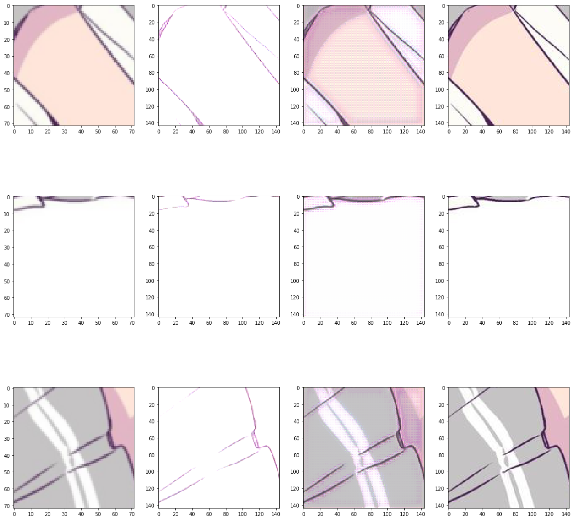
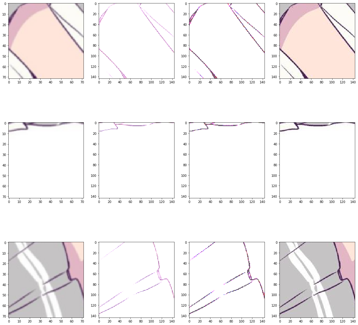
这是训练的最好的一次,最左侧是输入的模糊图片,第二列是网络的输出,第三列是做了直方图匹配得到的图片,第四列是ground truth。可以看到有很多小点点,我分析是tv loss占比太小的原因,当前tv loss乘以了0.1。于是将tv loss乘以0.5后又训练了一次,loss降到了58,结果如下:
感觉没法看了。。。

