CVPR 2016,大体原理:选择两张图片,一张作为风格图片,一张作为内容图片,任务是将风格图片中的风格,迁移到内容图片上。方法也比较简单,利用在ImageNet上训练好的VGG19,因为这种深层次的卷积神经网络的卷积核可以有效的捕捉一些特征,越靠近输入的卷积层捕捉到的信息层次越低,而越靠近输出的卷积层捕捉到的信息层次越高,因此可以用高层次的卷积层捕捉到的信息作为对风格图片风格的捕捉。而低层次的卷积层用来捕捉内容图片中的内容。所以实际的操作就是,将内容图片扔到训练好的VGG19中,取出低层次的卷积层的输出,保存起来,然后再把风格图片放到VGG19中,取出高层次的卷积层的输出,保存起来。然后随机生成一张图片,扔到VGG19中,将刚才保存下来的卷积层的输出的那些卷积层的结果拿出来,和那些保存的结果做个loss,然后对输入的随机生成的图片进行优化即可。原文链接:Image Style Transfer Using Convolutional Neural Networks
Image Style Transfer Using Convolutional Neural Networks
大体原理
选择两张图片,一张作为风格图片,一张作为内容图片,任务是将风格图片中的风格,迁移到内容图片上。方法也比较简单,利用在ImageNet上训练好的VGG19,因为这种深层次的卷积神经网络的卷积核可以有效的捕捉一些特征,越靠近输入的卷积层捕捉到的信息层次越低,而越靠近输出的卷积层捕捉到的信息层次越高,因此可以用高层次的卷积层捕捉到的信息作为对风格图片风格的捕捉。而低层次的卷积层用来捕捉内容图片中的内容。所以实际的操作就是,将内容图片扔到训练好的VGG19中,取出低层次的卷积层的输出,保存起来,然后再把风格图片放到VGG19中,取出高层次的卷积层的输出,保存起来。然后随机生成一张图片,扔到VGG19中,将刚才保存下来的卷积层的输出的那些卷积层的结果拿出来,和那些保存的结果做个loss,然后对输入的随机生成的图片进行优化即可。(Fig2)
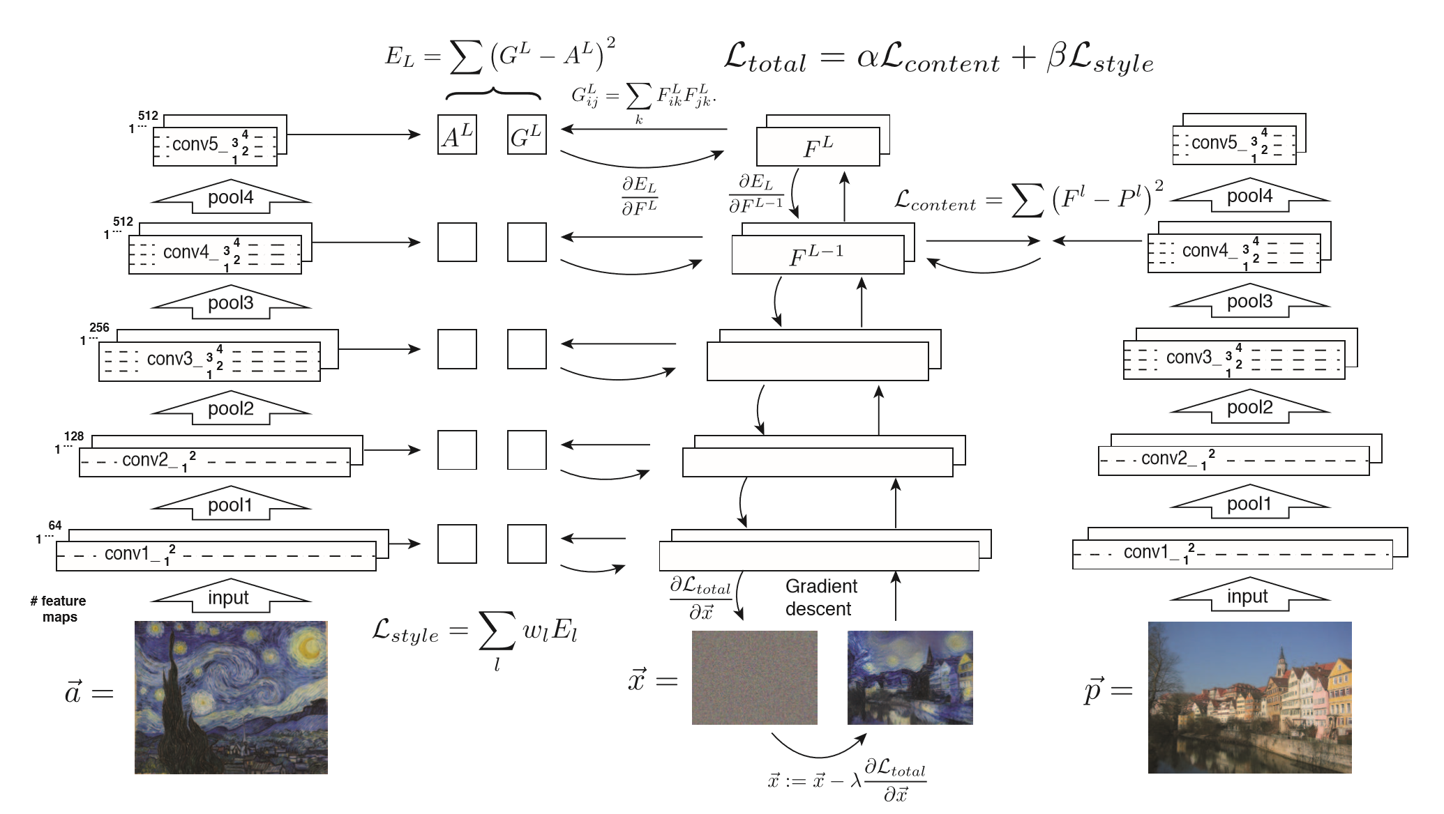
Figure 2. Style transfer algorithm. First content and style features are extracted and stored. The style image $\vec{a}$ is passed through the network and its style representation $A^l$ on all layers included are computed and stored(left). The content image $\vec{p}$ is passed through the network and the content representation $P^l$ in one layer is stored(right). Then a random white noise image $\vec{x}$ is passed through the network and its style features $G^l$ and content features $F^l$ are computed. On each layer included in the style representation, the element-wise mean squared difference between $G^l$ and $A^l$ is computed to give the style loss $\mathcal{L}_{style}$(left). Also the mean squared difference between $F^l$ and $P^l$ is computed to give the content loss $\mathcal{L}_{content}(right)$. The total loss $\mathcal{L}_{total}$ is then a linear combination between the content and the style loss. Its derivative with respect to the pixel values can be computed using error back-propagation(middle). This gradient is used to iteratively update the image $\vec{x}$ until it simultaneously matches the style features of the style image $\vec{a}$ and the content features of the content image $\vec{p}$(middle, bottom).
Deep image representations
We used the feature space provided by a normalized version of the 16 convolutional and 5 pooling layers of the 19-layer VGG network. We normalized the network by scaling the weights such that the mean activation of each convolutional filter over images and positions is equal to one. Such re-scaling can be done for the VGG network without changing its output, because it contains only rectifying linear activation functions and no normalization or pooling over feature maps. 其实这里我不是很明白为什么不会影响输出。
content representation
A layer with $N_l$ distinct filters has $N_l$ feature maps each of size $M_l$, where $M_l$ is the height times the width of the feature map. So the responses in a layer $l$ can be stored in a matrix $F^l \in \mathcal{R}^{N_l \times M_l}$ where $F^l_{ij}$ is the activation of the $i^{th}$ filter at position $j$ in layer $l$. Let $\vec{p}$ and $\vec{x}$ be the original image and the image that is generated, and $P^l$ and $F^l$ their respective feature representation in layer $l$. We then define the squared-error loss between the two feature representations
$$\mathcal{L}\_{content}(\vec{p}, \vec{x}, l) = \frac{1}{2}\sum\_{i, j}(F^l\_{ij}-P^l\_{ij})^2$$The derivative of this loss with respect to the activations in layer $l$ equals
\begin{equation} \frac{\partial{\mathcal{L}{content}}}{\partial{F^l{ij}}}=\left{ \begin{aligned} & (F^l - P^l){ij} & if \ F^l{ij} > 0 \ & 0 & if \ F^l_{ij} < 0 \end{aligned} \right. \end{equation}
from which the gradient with respect to the image $\vec{x}$ can be computed using standard error back-propagation.
When Convolutional Neural Networks are trained on object recongnition, they develop a representation of the image that makes object information increasingly explicit along the processing hierarchy. Higher layers in the network capture the high-level content in terms of objects and their arrangement in the input image but do not constrain the exact pixel values of the reconstruction very much. We therefore refer to the feature responses in higher layers of the network as the content representation.
style representation
To obtain a representation of the style of an input image, we use a feature space designed to capture texture information. This feature space can be built on top of the filter responses in any layer of the network. It consists of the correlations between the different filter responses, where the expecation is taken over the spatial extent of the feature maps. These feature correlations are given by the Gram matrix $G^l \in \mathcal{R}^{N_l \times N_l}$, where $G^l_{ij}$ is the inner product between the vecotrized feature maps $i$ and $j$ in layer $l$:
$$G^l\_{ij}=\sum\_kF^l\_{ik}F^l\_{jk}.$$By inducing the feature corelations of multiple layers, we obtain a stationary, multi-scale representation of the input image, which captures its texture information but not the global arrangement. Again, we can visualise the information captured by these style feature spaces built on different layers of the network by constructing an image that matches the style representation of a given input image. This is done by using gradient descent from a white noise image to minimise the mean-squared distance between the entries of the Gram matrices from the original image and the Gram matrices of the image to be generated. Let $\vec{a}$ and $\vec{x}$ be the original image and the image that is generated, and $A^l$ and $G^l$ their respective style representation in layer $l$. The contribution of layer $l$ to the toal loss is then
$$E\_l = \frac{1}{4N^2\_lM^2\_l}\sum\_{i,j}(G^l\_{ij} - A^l\_{ij})^2$$and the total style loss is
$$\mathcal{L}\_{style}(\vec{a}, \vec{x})=\sum^L\_{l=0}w\_lE\_l,$$where $w_L$ are weighting factors of the contribution of each layer to the total loss (see below for specific values of $w_l$ in our results). The derivative of $E_l$ with respect to the activations in layer $l$ can be computed analytically:
\begin{equation} \frac{\partial{E_l}}{\partial{F^l_{ij}}}=\left{ \begin{aligned} & \frac{1}{N^2_lM^2_l}((F^l)^T(G^l-A^l)){ji} & if \ F^l{ij} > 0 \ & 0 & if \ F^l_{ij} < 0 \end{aligned} \right. \end{equation} The gradient of $E_l$ with respect to the pixel values $\vec{x}$ can be readily computed using standard error back-propagation.
style transfer
To transfer the style of an artwork $\vec{a}$ onto a photograph $\vec{p}$ we synthesise a new image that simultaneously matches the content representation of $\vec{p}$ and the style representation of $\vec{a}$. Thus we jointly minimise the distance of the feature representations of a white noise image fron the content representation of the photograph in one layer and the style representation of the painting defined on a numebr of layers of the Convolutional Neural Network. The loss function we minimise is
$$\mathcal{L}\_{total}(\vec{p}, \vec{a}, \vec{x})=\alpha \mathcal{L}\_{content}(\vec{p}, \vec{x}) + \beta \mathcal{L}\_{style}(\vec{a}, \vec{x})$$where $\alpha$ and $\beta$ are the weighting factors for content and style reconstruction, respectively. The gradient with respect to the pixel values $\frac{\partial{\mathcal{L}_{total}}}{\partial{\vec{x}}}$ can be used as input for some numerical optimisation strategy. Here we use L-BFGS, which we found to work best for image synthesis. To extract image information on comparable scales, we always resized the style image to the same size as the content image before computing its feature representations.
Results
Trade-off between content and style matching
Since the loss function we minimise during image synthesis is a linear combination between the loss functions for content and style respectively, we can smoothly regulate the emphasis on either reconstructing the content or the style(Fig4).
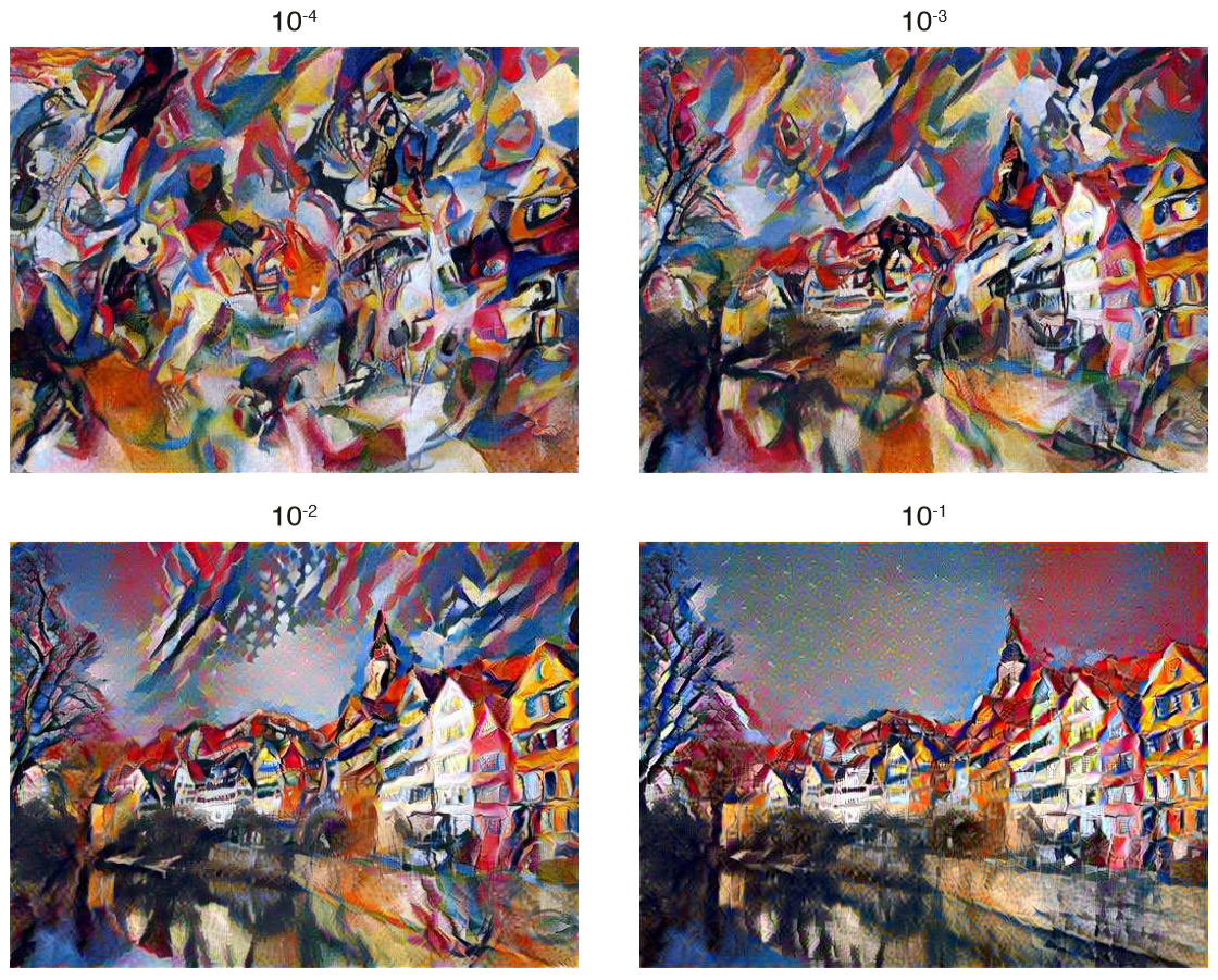 Figure 4. Relative weighting of matching content and style of the respective source images. The ratio $\alpha / \beta$ between matching the content and matching the style increases from top left to bottom right. A high emphasis on the style effectively produces a texturised version of the style image(top left). A high emphasis on the content produces an image with only little stylisation(bottom right). In practice one can smoothly interpolate between the two extremes.
Effect of different layers of the Convolutional Neural Network
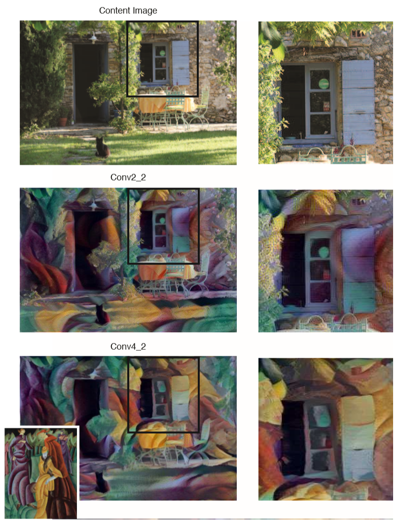 Figure 5. The effect of matching the content representation in different layers of the network. Matching the content on layer ‘conv2_2’ preserves much of the fine structure of the original photograph and the synthesised image looks as if the texture of the painting is simply blended over the photograph(middle). When matching the content on layer ‘conv4_2’ the texture of the painting and the content of the photograph merge together such that the content of photograph is displayed in the style of the painting(bottom). Both images were generated with the same choice of parameters($\alpha / \beta = 1 \times 10^{-3}$). The painting that served as the style image is shown in the bottom left corner and is name Jesuiten Ⅲ by Lyonel Feininger, 1915.
Another important factor in the image synthesis process is the choice of layers to match the content and style representation on. As outlined above, the style representation is a multi-scale representation that includes multiple layers of the neural network. The number and position of these layers determines the local scale on which the style is matched, leading to different visual experiences. We find that matching the style representations up to higher layers in the network preserves local images structures an increasingly large scale, leading to a smoother and more continuous visual experience. Thus, the visually most appealing images are usually created by matching the style representation up to high layers in the network, which is why for all images shown we match the style features in layers ‘conv1_1’, ‘conv2_1’, ‘conv3_1’, ‘conv4_1’and ‘conv5_1’ of the network.
To analyse the effect of using different layers to match the content features, we present a style transfer result obtained by stylising a photograph with the same artwork and parameter configuration ($\alpha / \beta = 1 \times 10^{-3}$), but in one matching the content features on layer ‘conv2_2’ and in the other on layer ‘conv4_2’(Fig5). When matching the content on a lower layer of the network, the algorithm matches much of the detailed pixel information in the photograph and the generated image appears as if the texture of the artwork is merely blended over the photograph(Fig5, middle). In contrast, when matching the content features on a higher layer of the network, deatiled pixel information of the photograph is not as strongly constraint and the texture of the artwork and the content of the photograph are properly merged. That is, the fine structure of the image, for example the edges and colour map, is altered such that it agrees with the style of the artwork while displaying the content of the photograph(Fig5, bottom).
Figure 5. The effect of matching the content representation in different layers of the network. Matching the content on layer ‘conv2_2’ preserves much of the fine structure of the original photograph and the synthesised image looks as if the texture of the painting is simply blended over the photograph(middle). When matching the content on layer ‘conv4_2’ the texture of the painting and the content of the photograph merge together such that the content of photograph is displayed in the style of the painting(bottom). Both images were generated with the same choice of parameters($\alpha / \beta = 1 \times 10^{-3}$). The painting that served as the style image is shown in the bottom left corner and is name Jesuiten Ⅲ by Lyonel Feininger, 1915.
Another important factor in the image synthesis process is the choice of layers to match the content and style representation on. As outlined above, the style representation is a multi-scale representation that includes multiple layers of the neural network. The number and position of these layers determines the local scale on which the style is matched, leading to different visual experiences. We find that matching the style representations up to higher layers in the network preserves local images structures an increasingly large scale, leading to a smoother and more continuous visual experience. Thus, the visually most appealing images are usually created by matching the style representation up to high layers in the network, which is why for all images shown we match the style features in layers ‘conv1_1’, ‘conv2_1’, ‘conv3_1’, ‘conv4_1’and ‘conv5_1’ of the network.
To analyse the effect of using different layers to match the content features, we present a style transfer result obtained by stylising a photograph with the same artwork and parameter configuration ($\alpha / \beta = 1 \times 10^{-3}$), but in one matching the content features on layer ‘conv2_2’ and in the other on layer ‘conv4_2’(Fig5). When matching the content on a lower layer of the network, the algorithm matches much of the detailed pixel information in the photograph and the generated image appears as if the texture of the artwork is merely blended over the photograph(Fig5, middle). In contrast, when matching the content features on a higher layer of the network, deatiled pixel information of the photograph is not as strongly constraint and the texture of the artwork and the content of the photograph are properly merged. That is, the fine structure of the image, for example the edges and colour map, is altered such that it agrees with the style of the artwork while displaying the content of the photograph(Fig5, bottom).
Initialisation of gradient descent
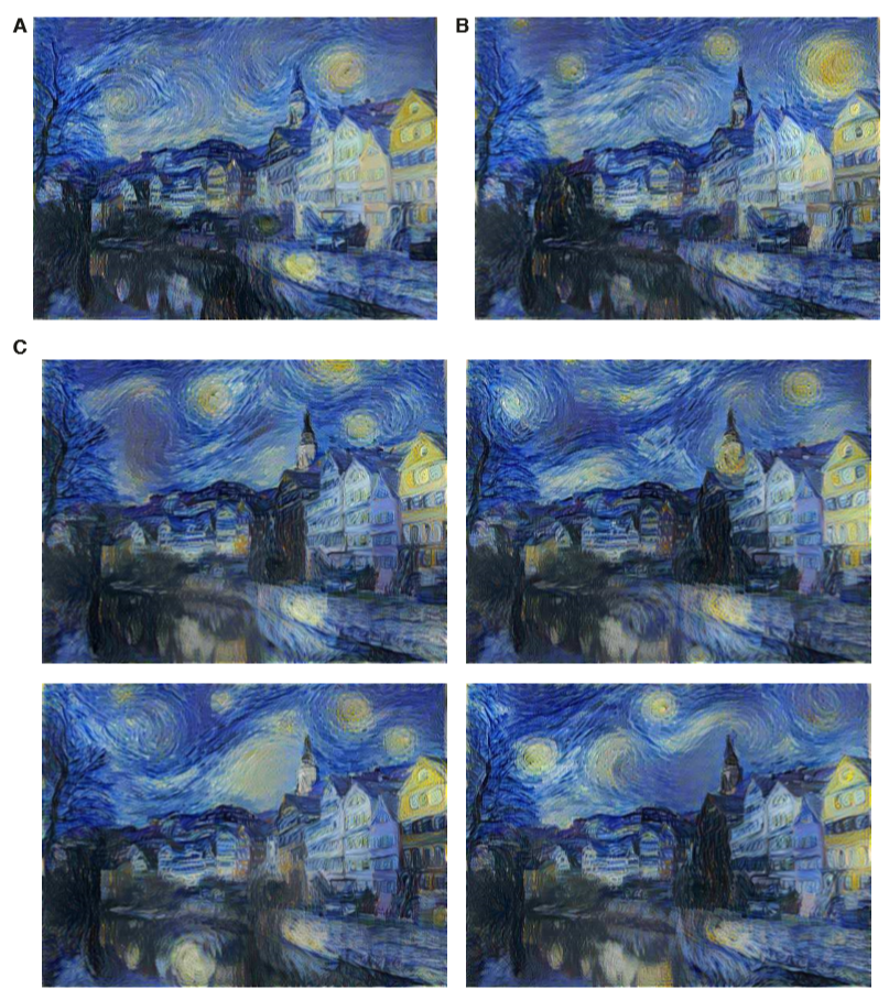 Figure 6. Initialisation of the gradient descent. A Initialised from the content image. B Initialised from the style image. C Four samples of images initialised from different white noise images. For all images the ratio $\alpha / \beta$ was equal to $1 \times 10^{-3}$
We have initialised all images shown so far with white noise. However, one could also initialise the image synthesis with either the content image or the style image. We explored these two alternatives(Fig6 A, B): although they bias the final image somewhat towards the spatial structure of the initialisation, the different intialisation do not seem to have a strong effect on the outcome of the synthesis procedure. It should be noted that only initialising with noise allows to generate an arbitrary number of new images(Fig6 C). Initialising with a fixed image always deterministically leads to the same outcome (up to stochasticity in the gradient descent procedure).
Figure 6. Initialisation of the gradient descent. A Initialised from the content image. B Initialised from the style image. C Four samples of images initialised from different white noise images. For all images the ratio $\alpha / \beta$ was equal to $1 \times 10^{-3}$
We have initialised all images shown so far with white noise. However, one could also initialise the image synthesis with either the content image or the style image. We explored these two alternatives(Fig6 A, B): although they bias the final image somewhat towards the spatial structure of the initialisation, the different intialisation do not seem to have a strong effect on the outcome of the synthesis procedure. It should be noted that only initialising with noise allows to generate an arbitrary number of new images(Fig6 C). Initialising with a fixed image always deterministically leads to the same outcome (up to stochasticity in the gradient descent procedure).
implementation
关于实现的部分,我自己用mxnet实现了一下,但是发现和mxnet的example里面给的非常不一样。在他们的实现里面提到了Total variation denoising。而且,论文中的loss function是sum of square,而图2中给出是MSE,取了个平均值。我实现是时候没有取平均,导致loss很大,但是也可以训练。但是自己实现的梯度下降很难收敛,需要对梯度进行归一化,后来使用MXNet的gluon的Trainer训练会比原来好很多。
Total variation denoising
In signal processing, total variation denoising, also known as total variation regularization, is a process, most often used in digital image processing, that has applications in noise removal.
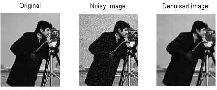 Example of application of the Rudin et al.[1] total variation denoising technique to an image corrupted by Gaussian noise. This example created using demo_tv.m by Guy Gilboa, see external links.
It is based on the principle that signals with excessive and possibly spurious detail have high total variation, that is, the integral of the absolute gradient of the signla is high. According to this principle, reducing the total variation of the signal subject to it being a close match to the original signal, removes unwanted detail whilst preserving important details such as edges. The concept was pioneered by Rudin, Osher, and Fatemi in 1992 and so is today known as the ROF model.
This noise removal technique has advantages over simple techniques such as linear smoothing or median filtering which reduce noise but at the same time smooth away edges to a greater or lesser degree. By contrast, total variation denoising is remarkably effective at simultaneously preserving edges whilst smoothing away noise in flat regions, even at low signal-to-noise ratios.
Example of application of the Rudin et al.[1] total variation denoising technique to an image corrupted by Gaussian noise. This example created using demo_tv.m by Guy Gilboa, see external links.
It is based on the principle that signals with excessive and possibly spurious detail have high total variation, that is, the integral of the absolute gradient of the signla is high. According to this principle, reducing the total variation of the signal subject to it being a close match to the original signal, removes unwanted detail whilst preserving important details such as edges. The concept was pioneered by Rudin, Osher, and Fatemi in 1992 and so is today known as the ROF model.
This noise removal technique has advantages over simple techniques such as linear smoothing or median filtering which reduce noise but at the same time smooth away edges to a greater or lesser degree. By contrast, total variation denoising is remarkably effective at simultaneously preserving edges whilst smoothing away noise in flat regions, even at low signal-to-noise ratios.
1D signal series
For a digital signal $y_n$, we can, for example, define the total variation as:
$$V(y)=\sum\_n\vert y\_{n+1}-y\_n\vert$$Given an input signal $x_n$, the goal of total variation denoising is to find an approximation, call it $y_n$, that has smaller total variation than $x_n$ but is “close” to $x_n$. One measure of closeness is the sum of square errors:
$$E(x, y)=\frac{1}{2}\sum\_n(x\_n - y\_n)^2$$So the total variation denoising problem amounts to minimizing the following discrete functional over the signal $y_n$:
$$E(x, y) + \lambda V(y)$$By differentiating this functional with respect to $y_n$, we can derive a corresponding Euler-lagrange equation, that can be numerically integrated with the original signal $x_n$ as initial condition. This was the original approach. Alternatively, since this is a convex functional, techniques from convex optimization can be used to minimize it and find the solution $y_n$.
Regularization properties
The regularization parameter $\lambda $ plays a critical role in the denoising process. When $\lambda = 0$, there is no smoothing and the result is the same as minimizing the sum of squares. As $\lambda \to \infty $, however, the total variation term plays an increasingly strong role, which forces the result to have smaller total variation, at the expanse of being less like the input (noisy) signal. Thus, the choice of regularization parameter is critical to achieving just the right amount of noise removal.
2D signal images
We now consider 2D signals $y$, such as images. The total variation norm proposed by the 1992 paper is
$$V(y) = \sum\_{i,j}\sqrt{\vert y\_{i+1,j}-y\_{i,j}\vert ^2 + \vert y\_{i, j+1} - y\_{i, j}\vert ^2}$$and is isotropic and not differentiable. A variation that is sometimes used, since it may sometimes be easier to minimize, is an anisotropic version
$$V\_{aniso}(y) = \sum\_{i,j}\sqrt{\vert y\_{i+1,j}-y\_{i,j}\vert ^2} + \sqrt{\vert y\_{i,j+1} - y\_{i,j}\vert ^2} = \sum\_{i,j}\vert y\_{i+1,j}-y\_{i,j}\vert + \vert y\_{i,j+1}-y\_{i,j}\vert $$The standard total variation denoising problem is still of the form
$$\min\_yE(x,y)+\lambda V(y)$$where $E$ is the 2D L2 norm. In contrast to the 1D case, solving this denoising is non-trivial. A recent algorithm that solves this is known as the primal dual method. Due in part to much research in compressed sensing in the mid-2000s, there are many algorithms, such as the split-Bregman method, that solve variants of this problem.
不过我个人在实现的时候,实现了两个版本,一个是增加了total variation denoising,另一个是没增加total variation denoising的a。 代码如下:
| |
这里在实现的时候,使用了这个2D图像的total variation denoising,也就是,每个像素应尽可能的与左侧和上方的像素相近。所以最后的优化目标是三部分组成,第一部分是content loss,第二部分是style loss,第三部分是total variation loss。 研究一下mxnet给出的example model_vgg19.py
| |
nstyle.py
| |